Tutorial

Author

Khaya Donald Mpehle, Steven Maharaj

Here we will introduce a python library, GaussRF, concerned with simulating Gaussian Random fields in one-dimension and two-dimensional rectangular domains. The library will implement two sampling methods, one approximate and one exact. The Karhunen-Loève expansion, using the Nyström method to solve further numerical problems, is the approximate method, while the circulant embedding method is the exact sampling procedure. The document is structured as follows: a brief discussion on the theory random fields will start. The main part of the document will then introduce the key functions in GaussRF and give examples of their use. The document will finish by listing expansions to this library that should be prioritized.

The Karhunen Loève approximation

Let \(X_t\) be a zero mean Gaussian field, where \(t \in T\), with covariance function

\[R(t,s) = E\left[X_tX_s\right].\]

The Karhunen-Loève expansion theorem states that \(X_t\) can be expanded as

\[X_t = \sum_{k=1}^\infty \sqrt{\lambda_k}Z_k \phi_k(t).\]

In this expansion \(Z_k\) are iid standard normal variables while \(\phi_k\) and \(\lambda_k\) are respectively the eigen-functions and -values of the RF’s covariance function. Therefore \(\phi_k\) and \(\lambda_k\) satisfy the eigenvalue problem

\[\int_{t\in T} R(t,s)\phi_k(s)ds = \lambda_k\phi_k(t)\]

The Karhunen-Loève expansion can roughly be thought of as “separating” the deterministic and random components of the Gaussian RF. A means of approximating the RF \(X_t\) is to truncate the KL expansion after \(N\) terms. This is termed the Karhunen-Loève approximation of order \(N\). With a finite number of terms in the expansion, the only remaining task is to find the eigenvalues and -functions of the convariance function. There are several ways to do this, here we shall focus on using the Nyström method [1,4]. The integral eigenvalue problem (3) is approximated by an M-point quadrature \(\{w_i,x_i\}_{i=1}^M\), the resulting expression is considered on each of the quadrature points:

\[\sum_{i=1}^M w_i R(t_j,s_i) \phi_k(s_i) = \lambda_k \phi(t_j),\hspace{7mm} j=0,1,2,\ldots,M.\]

The discrete expression (4) reduces to the matrix eigenvalue problem

\[\mathbf{C}\bf{W}\mathbf{\phi}_k = \lambda_k \mathbf{\phi}_k\]

where we have introduced the diagonal matrix of weights \(\mathbf{W} = \text{diag}\{w_1,\ldots,w_M\}\) and the covariance matrix \((\mathbf{C})_{ij} = R(t_i,t_j)\). Solving this eigenvalue problem will determine the eigenvectors and -values of the discretised system of (3) and allow the determination of the discrete KL approximation. We note as a practical consideration that (5) can be modified by left multiplying both sides by \(\mathbf{W}^{1/2}\), such that the system

\[\mathbf{W}^{1/2}\mathbf{C}\mathbf{W}^{1/2}\mathbf{y}_k = \lambda_k \mathbf{y}_k,\]

where \(\mathbf{y}_k = \mathbf{W}^{1/2}\mathbf{\phi}_k\), is obtained. This system is advantageous as \(\mathbf{W}^{1/2}\mathbf{C}\mathbf{W}^{1/2}\) is a positive semi-definite symmetric matrix and therefore has orthogonal eigenvectors with positive,real eigen values.

Examples

We have produced code using python and its numpy library to compute the Karhunen-Loève expansion on one- and two-dimensional rectangular domains.There are two quadrature methods implemented so far. The first is the “EOLE” method in which the quadrature points \(x_i\) are evenly spaced and the weights \(w_i = |\Omega|/N\) are equal. The second is the Gauss-Legendre quadrature where the quadrature points used are those of the Gauss-Legendre quadrature.

The function KL1DNys will return a simulation of the Gaussian process \(X_t\) when given its covariance function \(R(t,s)\). In figure 1, the eigenvalues of the Brownian motion process along with the first six eigenfunctions, which have analytical solutions, are compared to our EOLE Nyström simulation. One can see good agreement between the exact eigenvalues and our numerical approximation.

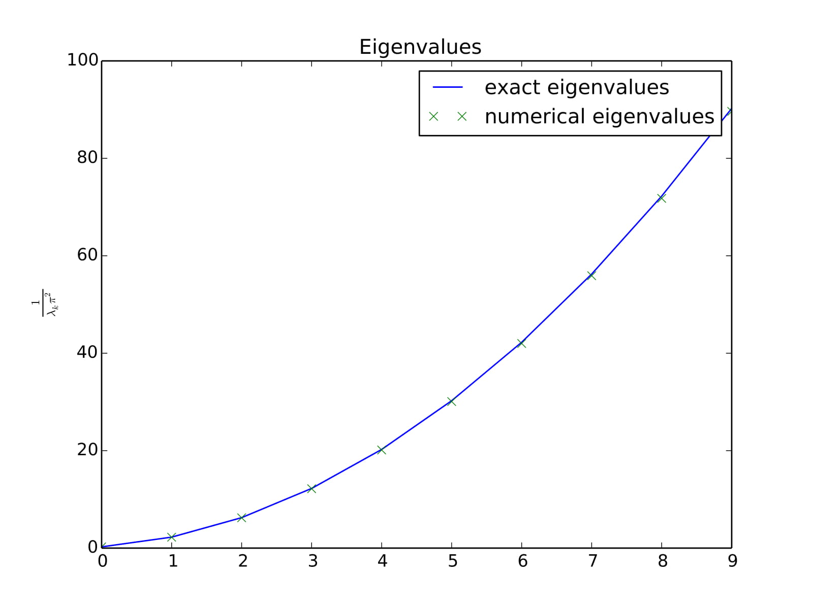
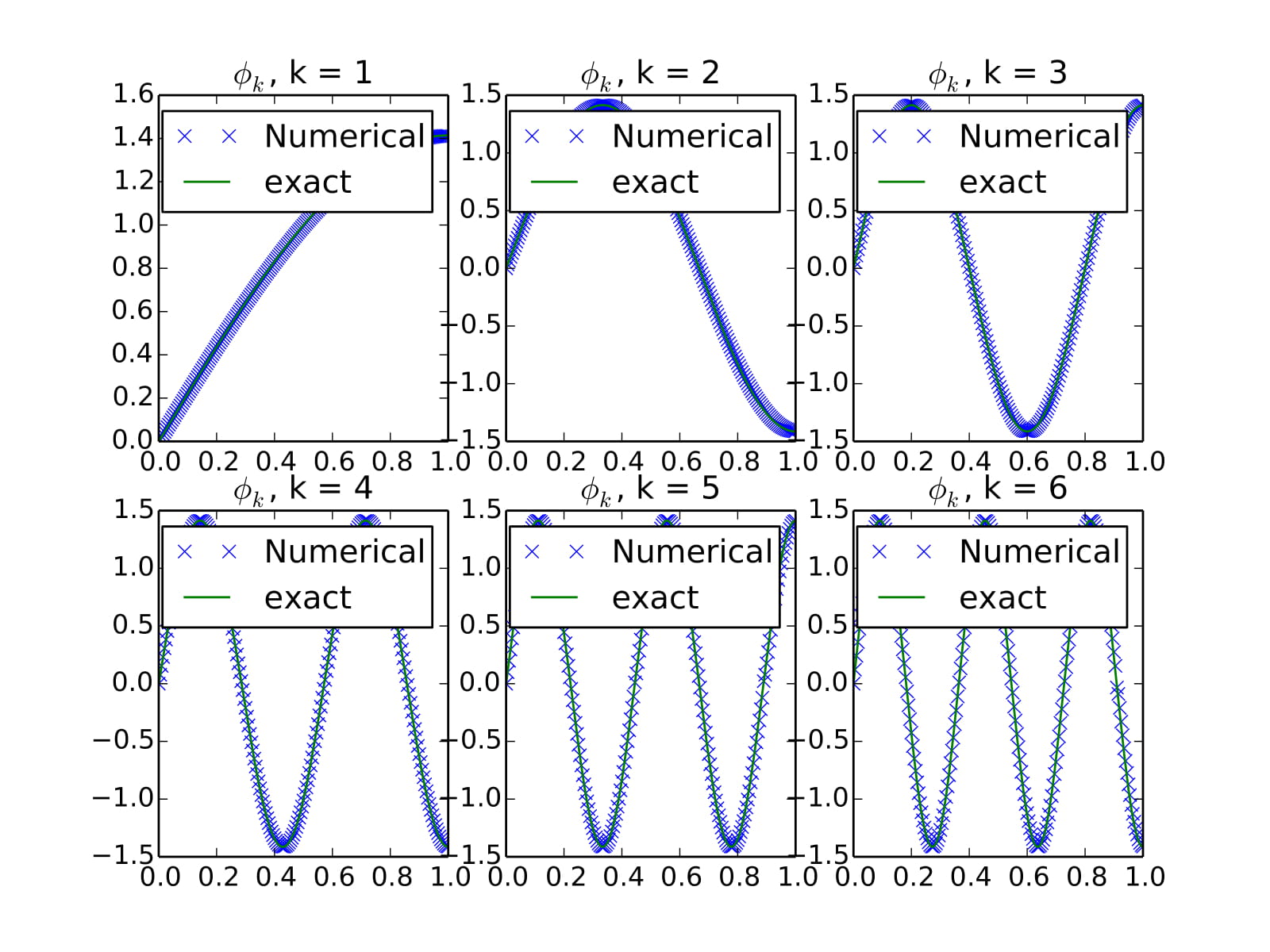
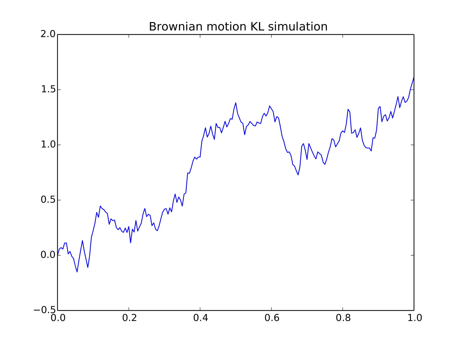
Top: Comparison of the numerical eigenvalues to the exact eigenvalues in the Brownian motion Karhunen-Loève function expansion.Middle: Comparison of the exact and numerical 5th eigenfunction. Bottom: The approximate Brownian motion in an \(N=200\) term expansion. Here N=200 quadrature points were used.

The function KL2DNys will return a simulation of the Gaussian field \(X_t\), \(t\in \mathbb{R^2}\) with supplied covariance function, on a rectangular domain. As an example, consider the Gaussian RF with the stationary, isotropic exponential covariance given by

\[R(s,t) = \exp\left( - \frac{|s - t ||}{\rho} \right)\]

where \(\rho\) is some scale radius. In figure 2, we see a plot of the eigenvalues of this covariance matrix along with the first 5 eigenfunctions, simulated on the domain \([0,1] \times [0,1]\) with \(50 \times 50\) points. Note that this is a small number of simulation points to be using, but this is all that the the relatively weak computer’s RAM allows to be used. This is a limitation of our current resources, and a full convergence test with finer discretisations, on a more powerful computer, is called for.

Top: Eigenvalues of the 2D exponential covariance function Gaussian RF. Middle: The first 6 eigenfunctions. Bottom: The random field realisation. There are \(50 \times 50\) points and the order of the expansion is \(N = 100\).

Circulant Embedding methods

Suppose \(X_t\) is a stationary Gaussian random field so that its covariance function is of the form \(R(s,t) = R(s-t)\). In such a case, it may be preferable to use the Circulant Embedding Method. The method is so-called because it exploits the fact that the covariance matrix of stationary SPs can be embedded into a larger circulant matrix. Then one can use the Fast Fourier Transform to compute the eigenvalues of the circulant matrix, and from there go on to simulate the RF. The details of the method are described in [2,3]. What is desirable about the Circulant Embedding algorithm is its generation of a sample that has the exact covariance structure, and its speed. The function circembed1D.py will return an array containing the simulated Gaussian process when given a power of two g, the end points a, b of the domain and the covariance function. 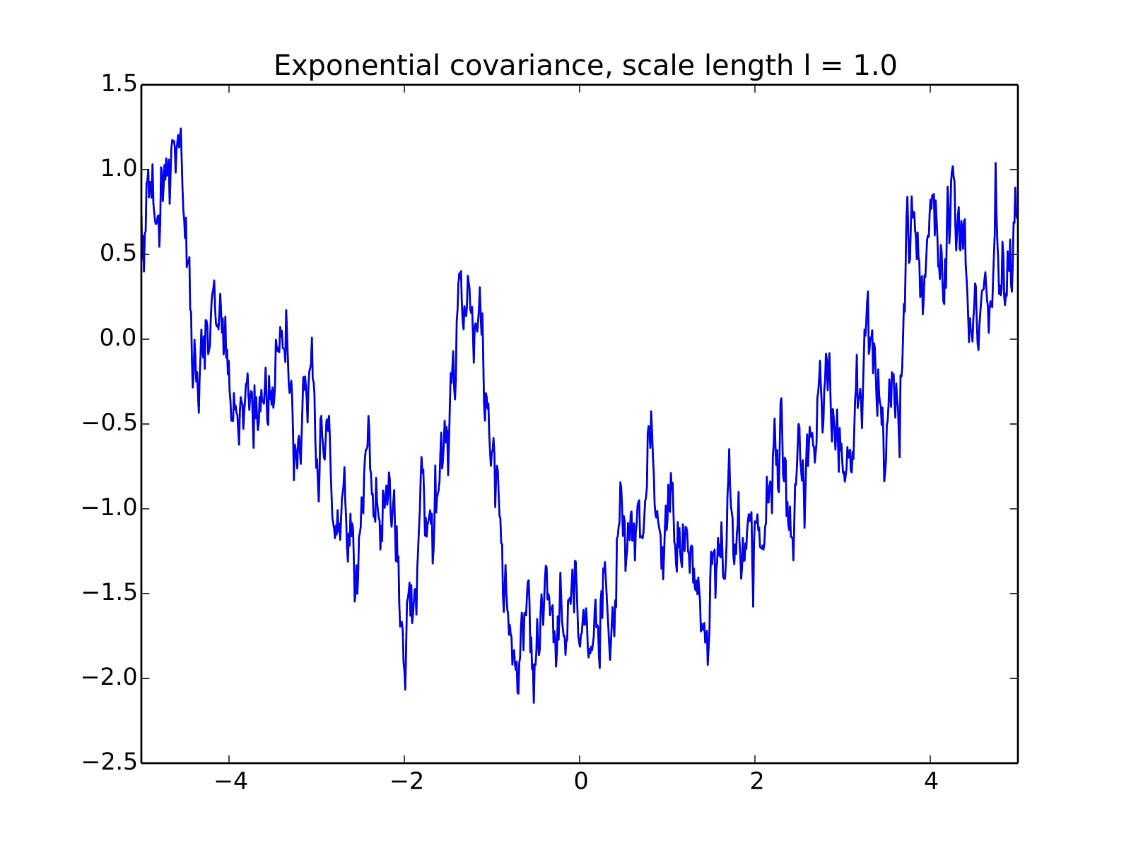The sample size will be \(N = 2^g\), as the Circulant Embedding method requires the sample size to be a power of two to be efficient. In figure 3 we plot a realisation of the SP with the exponential covariance function

\[R(s,t) = R(s-t) = \exp\left(\frac{|s-t|}{l}\right).\]

A similar function circembed2D.py implements the method in two-dimensions. The method will produce a Gaussian Random field. As an example, we take an example given in Newsam and Dietrich, the Gaussian RF with the covariance

\[R(s,t) = \exp \left( (s-t)^T A (s-t)\right)\]

where \(A\) is the positive-definite, symmetric matrix

\[\begin{split}A =\left( \begin{array}{cc} 3 & 1 \\ 1 & 2 \end{array} \right).\end{split}\]

Top: A Realisation of the 1-D exponential random process.Bottom: A realisation of the 2D homogeneous Gaussian RF with anisotropic covariance (9).

Extensions

We list here extensions to the library of functions that should be prioritised. In no particular order we should add functions to:

• Implement the Cholesky decomposition simulation procedure in one- and two-dimensions

• Implement Galerkin projection methods in one- and two-dimensions[1].

  • In particular, we should implement Haar-wavelet basis functions[5] due to the potential of a speed boost compared to other finite-element basis functions.

• Add features for spatial statistics

Bibliography

[1] Betz, W., Papaioannou, I., & Straub, D.(2014). Numerical methods for the discretization of random fields by means of the Karhunen-loève expansion. Computer Methods in Applied Mechanics and Engineering,271, 109-129.

[2] Dietrich, C. R., & Newsam, G. N. (1993). A fast and exact method for multidimensional Gaussian stochastic simulations. Water Resources Research, 29(8), 2861-2869.

[3] Chan, G., & Wood, A. T. (1999). Simulation of stationary Gaussian vector fields. Statistics and computing, 9(4), 265-268.

[4] Atkinson, K. E. (1967). The numerical solution of Fredholm integral equations of the second kind. SIAM Journal on Numerical Analysis, 4(3), 337-348.

[5] Phoon, K. K., Huang, S. P., & Quek, S. T. (2002). Implementation of Karhunen-Loeve expansion for simulation using a wavelet-Galerkin scheme. Probabilistic Engineering Mechanics, 17(3), 293-303.